Handout 2: Demand and Supply
31st August 2015

Competitive Markets and How They Work (Demand and Supply)
Eternal Economic Truth: attempts to fight market forces usually backfire.
The essence of any market is trade – somebody has to sell, and somebody must be willing to buy the product being offered. The market thus is a term used by economists to describe the process through which products, which are fairly similar, are bought and sold.
Demand
Demand relates to the buying side of the market, from the point of view of the consumer. Demand can be defined as the desire for a product backed up by the willingness and ability to pay for it. This describes a situation which is effective demand, because it relates to demand backed up by the ability to buy the good, this is important because companies are not interested in demand unless that person can buy the product.
For the sake of simplicity it is assumed that all other factors, except for price remain constant. This is known as the Ceteris Paribus assumption.
The table below can be used to plot a demand curve. This will show the number of Manchester United tickets demanded at a given price.
| Price of Man Utd tickets(£) | Quantity Demanded per game ‘000 | |
| £75 | 40 | |
| £65 | 50 | |
| £55 | 60 | |
| £45 | 70 | |
| £35 | 80 |
Table One
This can be illustrated in the diagram below.
Point to note
When price goes up, there is a decrease in the quantity demanded. When price goes down, there is an increase in 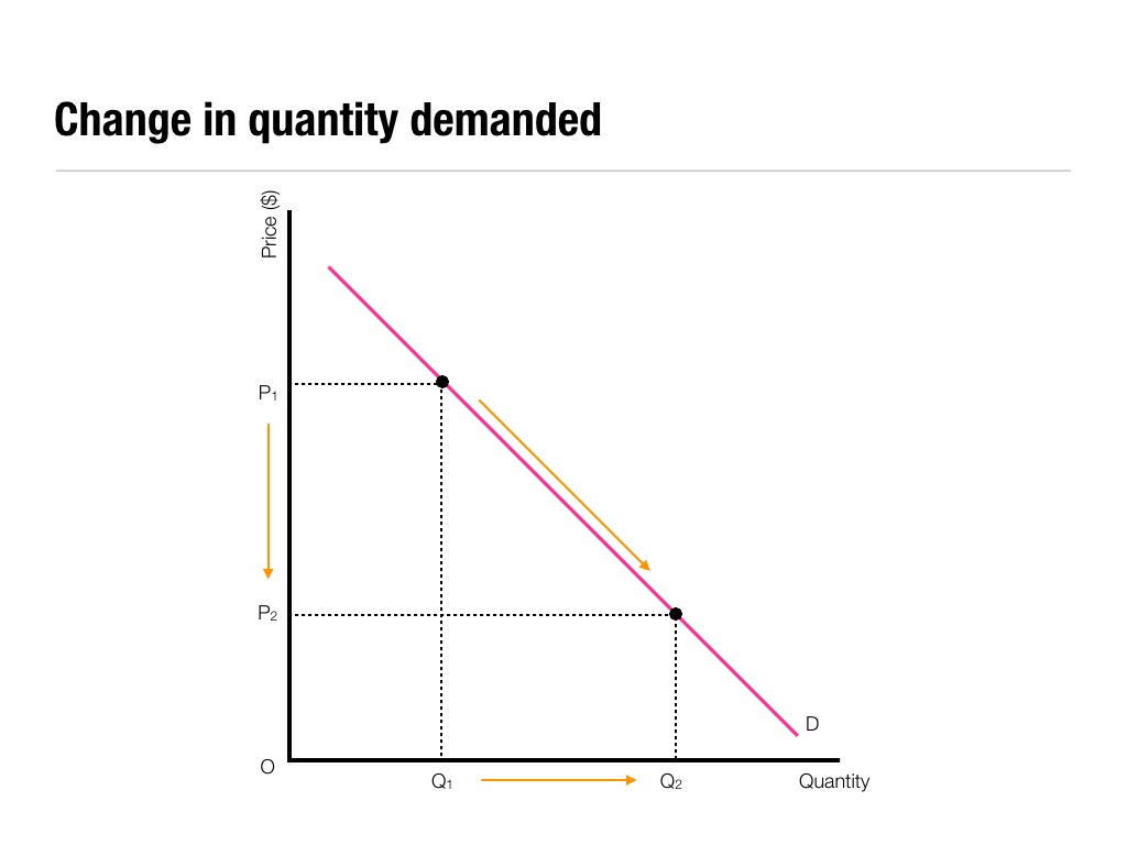 quantity demanded i.e. when there is a change in price there is an immediate change in quantity demanded.
We can also use these figures to illustrate the total expenditure by consumers on goods or services. In addition this shows us the level of revenue a firm gets at a given price. For example if the price is £55 then the demand curve suggests that Manchester United would sell 55000 tickets. The revenue or total expenditure would be £55 x 55000 = £3,025,000.
Consumer Surplus
Consumer Surplus occurs when consumers would be willing to pay more for a product than the actual price, apart from  the last unit purchased. In the diagram on the left, we again show a demand curve in red and add a supply curve in blue, which is a vertical line – there is a fixed supply of Man United tickets given by the stadium capacity of 75,000. Consumer surplus is the area above the price paid and below the demand curve i.e. the blue shaded in area at a price of P1. This can be illustrated by looking at the quantity demanded at points to the left of Q1. Some fans would be willing to pay more than P1 (the distance between the line P1 and the red demand curve), but only need to pay P1. There is a gain to some consumers of the area B. The biggest gain is to the Man United supporter willing to pay the price where the red line intersects the y axis.
Therefore if the price changes the consumer surplus will also change, if price was to rise the consumer surplus would contract, as the number of people willing to buy the product at the higher price will decline. Some consumers opt out of going to the game altogether.
What of area B? This represents the total revenue to Manchester United – the price x quantity sold. If they price to exactly fill the stadium, they need a price of £35 which yields £35 x 75,000 = £2,625,000 of revenue. Note that this is less revenue in this example than a ticket price of £55 – but a football club will not wish to irritate its fan base – even if this means sacrificing income in the short term. After all, the loyalest supporters may be the least able to pay higher prices.
Shifts in the Demand Curve
Price is not the only factor that can change, indeed changes in the ceteris paribus factors cause shifts in the demand curve. A shift to the right indicates an increase in demand at each and every price level. A shift to the left indicates a decline in demand at each and every price level.
Causes of Shifts in the Demand Curve
Generally shifts in the demand curve can be attributed to 3 factors.
- The financial ability to pay
- Attitude towards the product (which we call tastes, often influenced by advertising)
- Price, availability and quality of substitutes and complements.
Financial ability to pay
The ability to pay is clearly influenced by the amount of disposable income (after deducting tax and adding benefit) a person has, in addition to the ease with which a person can obtain loans or credit and the interest rate associated.
An increase in disposable income, or ease with which loans may be obtained, or decline in interest rates will increase an individual’s purchasing power causing the demand curve to shift to the right i.e. D1 to D3 in figure 6.
With most goods there is a positive relationship between income and product demand. So as income rises, demand rises, and vice versa. These goods are referred to as normal goods. However for some goods demand falls and income rises, for example the demand for black & white TVs has fallen as average incomes have risen. These goods are characterised by a negative relationship between income and demand, and are known as inferior goods.
Attitude towards the Product
People are clearly also influenced by individual desires, peer pressure and branding. These work to increase demand at each and every price for some goods, and also to reduce demand.
Price, availability and quality of Substitutes and Complements.
Substitute products are alternatives – products that are similar, and that satisfy the same wants and needs. The range of substitutes can be fairly narrow, for example in terms of different brands: JVC or Sony televisions. It can also be broad for example different type of music format: Vinyl, CD, Minidisc, Cassette or MP3. A rise in price will cause an increase in the demand for the substitute product.
Complements are products which go hand in hand with another product. For example roast beef and horseradish, turkey and cranberry sauce or tennis rackets and balls. A rise in price will cause a decline in demand for the main good, and as a result also for the complementary good.
Other factors which influence demand
Each product has unique factors that affect the demand for it. For example the demand for ice cream, or swimwear may be affected by the weather. If house prices or share prices are expected to rise in the future, this may cause demand to rise.
Supply
Supply refers to the quantity of a good or service a supplier is willing to make available for sale at a given price.
The profit motive is likely to be the major influence on company behaviour. The higher the price the more likely a firm is going to make increased profits.
The Supply Curve
The supply curve can represent the supply curve of one individual firm, or those of a number of firms representing the industry.
The supply curve is upward sloping. So an increase in the price that a product may be sold for would cause a firm to increase the amount of a good or service it offered for sale. As price falls, supply falls as the possibilities for profit decline.
Producer Surplus
Producer surplus is a gain from the viewpoint of the supplier.
In the diagram below, at prices between P1 the firm (or in a market supply, a number of firms) is willing to supply the market, but not to the same extent as at P1. At a price of 0 no units will be supplied. The producer surplus is the area between the upward-sloping supply curve and the price line from P1. It represents the excess revenue earned above the amount the firm needs to supply the product. Therefore although the firm (or in a market, the more efficient firms) is willing to accept a much lower price then P1, it is receiving this as payment, and thus a surplus exists.
Economic welfare is the sum of consumer and producer surpluses.
Shifts in the Supply Curve
Companies supply intentions are often influenced by more than just price, such factors can be illustrated by shifts in the supply curve. A shift to the right indicates an increase in supply, whilst a shift to the left signifies a decline in supply at each and every price.
There are 3 main causes of shifts in the supply curve
- Costs
- The size of the industry
- Legislation and taxation
Costs: Since the firm exists in a competitive market, it cannot exist indefinitely sustaining losses, companies will have to make decisions on how much to supply on the basis of the price they can get for selling the product.
If a factor of production rises in price, and so raises the costs of production, there is likely to be a shift to the left in the supply curve. From S1 to S2 in figure nine. If the factor of production falls in cost there is likely to be a shift to the right i.e. from S1 to S3
The size of the industry: If profits can be made in an industry it is clear that firms both in and outside the industry will react. Firms currently in the industry will invest to increase production, possibly by purchasing capital goods. Firms outside the industry may attempt to enter the industry and set-up businesses so as to take advantage of these profit opportunities. The ease with which new firms can establish in the industry is dependent upon the size of barriers to entry. However if the size of the industry grows, supply is also likely to increase. If firms now start to compete more the likely impact is that the supply curve will shift to the right as the firms compete away any profits that exist and reduce price.
Legislation and Taxation: Legislation designed to protect consumers or workers may impose additional costs upon companies, causing the supply curve to shift to the left. Government may impose indirect taxes, such as VAT, this can either result in an increase in price, or decline in supply at the given price as indicated by a shift in the supply curve to the left. On the other hand subsidies will increase and cause the supply curve to shift to the right.
Other factors influencing Supply
- Weather: In agricultural markets in particular this can influence the size of yields.
- Expectations: In markets such as the stock market, expectations of future performances can result in additional supply being made available by shareholders.
Bringing Demand & Supply together
Equilibrium refers in this instance to the point where demand and supply cross. In general it refers to a state of rest, where things do not have a tendency to change. In the diagram below this occurs at a price of P1.

If the market operated at P2, then the market would be in disequilibria, with supply outstripping demand at this high price. Thus a situation of excess supply would exist. The firm would thus not be selling all of its output and instead be adding to stocks. This would be irrational in the long-run, it is likely that firms would cut prices, and reduce their output. As the price starts to fall, more people are tempted back into the market, thus the gap between supply and demand narrow. This should eventually return to equilibrium, whether through analysis or guesswork.
If prices were set at P3, the market would again be faced with disequilibria, this time however demand is greater than supply, in other words excess demand exists. Consumers are keen to purchase what they consider to be bargains. Given the low price, supply is smaller than demand. However profit-seeking businesses will see these opportunities to sell more goods, and raise price whilst increasing supply. Once again the market would be expected to return to equilibrium.
Changes in Demand
If there is an increase in demand from D1 to D2, then at the original price of P1, there is a disequilibrium, with an excess demand equal to A- B. Suppliers will identify this opportunity and raise prices, and supply until equilibrium is returned to at a price of P2, with a higher quantity bought and sold.
Changes in Supply
If there is an increase in supply from S1 to S2 in Figure 12, then at the price P1 there is disequilibrium equal to C-E. Firms will find that stocks are building up, and so reduce price, eventually causing the market to return to equilibrium now at P2Q2.
Changes in Supply & Demand
In the diagram above, equilibrium is at a price of P1 where D1 and S1 cross. There is an increase in demand from D1 to D2, whilst simultaneously there is a shift in the supply curve S1 to S2, as a consequence the price remains unchanged, whilst the quantity bought and sold rises to Q2.
0 Comments