Handout: Short Run Production Theory
21st September 2015

http://www.slideshare.net/salasvelasco/microeconomics-production-theory
Production theory shows us how different combinations of factors produce a level of output in the short and long run. It helps explain how productivity performance, output per worker or Average Product (AP) crucially affects company costs. Remember our eternal economic truth : in the long run productivity growth is almost all that matters for economic health and wealth. Here we introduce the short run law of diminishing returns and the long run idea of returns to scale.
Inputs
The three factors of production give us three inputs which combine in some ratio in the production process. The three factors are land (La) Labour (L) and Capital, (K) which have three market prices, rent, wages and the rate of interest.
As a formula we can say
Qx = f(L, La, K)
Or in words, output Q of a product x is produced by a combination of land (La), labour (L) and capital (K).
The Short Run
The law of diminishing returns states that if increasing quantities of a variable factor (labour) are added to a fixed factor (capital) the average and marginal products will eventually diminish. So in the short run Capital is fixed. In our simple model, labour is the one variable factor, which we can plot against output to give a relationship – labour productivity.
Notice this is a short run law. The short run has nothing to do with time – it is defined simply as that period of activity where at least one factor is held constant.
In the real world, it takes time for firms to invest in new capital – machines or buildings. So in the long run we say all factors are variable – and the law of diminishing returns will no longer apply. As new technology is introduced there is no reason why factor productivity shouldn’t rise. We plot marginal product, average product and total product against output.
A numerical example
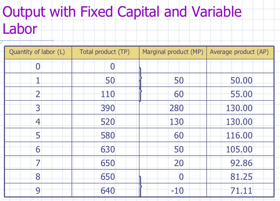
The table above shows the relationship between Total Product and Marginal Product. The Marginal Product measures the change in total product (output) as we add one more unit of labour (L).
The following “neoclassical” story explains how growth occurs. The change in technology is assumed to grow at a constant rate. At some point (worker 4) we can see that the marginal product begins to fall. And at the ninth worker it becomes negative.
Imagine we are adding workers to an assembly line. At some point the additional worker contributes less – the productivity or average product (AP) begins to fall. We cannot change the capital and invest in new machinery – that is fixed in quantity as it’s a short run scenario.
At nine workers they begin to get in each other’s way and the ninth worker actually has a negative impat on the production process – his contribution is less than zero. We can plot this relationship:
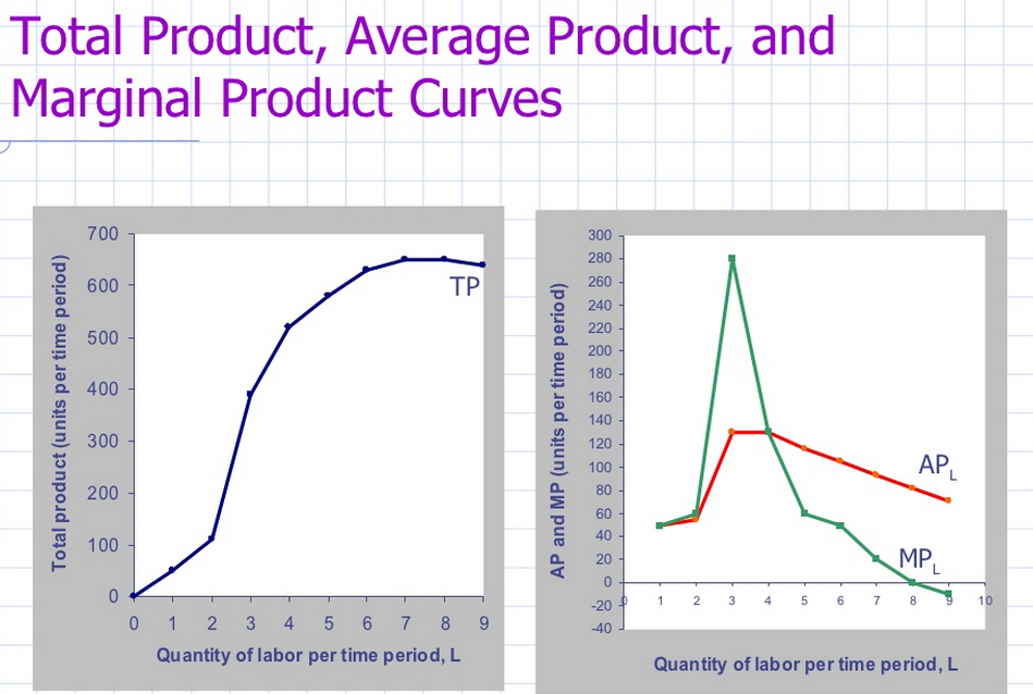
We can see visually how marginal product peaks at the third worker, and how productivity overall (AP begins to fall at worker 4. The productivity of this workforce is highest at three workers. And we can also illustrate a fundamental mathematical truth: where MP equals zero at 8 workers total output (TP) is at its highest point.
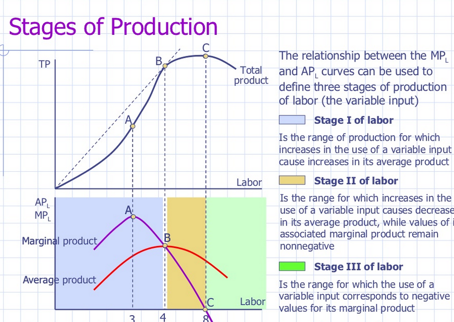
Stages of Short Run Production
We can use the same figures and graphs to illustrate how a firm’s production goes through three stages – increasing returns, diminishing returns and negative returns.
Two Equivalent Decision Rules for the Profit Maximising Firm
Hire L, the number of workers, such that the firm maximises profits. This occurs where
Maximum Value (Total Value of Output – Total Cost of Input) = Max Total Profit
Hire L so that the marginal revenue product, MRP, is equal the marginal cost, MC. That is…
MRP = MC where MRP = MP x Px (Px = output price)
Given the PX = Price of the output = £3, and the PL = price of the input, ie. labour = £600 a week, and the following input and marginal product information, the following relationships are derived. Assume additionally that each labourer is paid the same amount, that is, the input cost of each additional worker is the same, or the marginal cost of each worker is the same, thus PL = MCL = £600.
| (1)L | 2)Output | (3)MP | (4)P | (5) MRP | (6)Wage (MC of Labour) | (7)Additional Profit MRP -W |
| Labour | TP/L | £200 | Price x MP | £600 | (5) – (6) | |
| 0 | 0 | 0 | £200 | 0 | £600 | 0 |
| 1 | 6 | 6 | £200 | £1200 | £600 | £600 |
| 2 | 11 | 5 | £200 | £1000 | £600 | £400 |
| 3 | 16 | 4 | £200 | £800 | £600 | £200 |
| 4 | 18 | 3 | £200 | £600 | £600 | 0 |
| 5 | 20 | 2 | £200 | £400 | £600 | – £200 |
| 6 | 21 | 1 | £200 | £200 | £600 | – £400 |
The rational firm will hire the number of units, ie. workers, so that Total Profit is 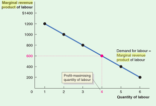 maximised, and the number of inputs so that the MRP = MCL. We can see that in the above table, this comes where £600 = £600, which is four workers. The marginal revenue product (or value this last worker contributes to profit) is zero. So it is rational to stop at hiring four workers. We can also illustrate this graphically and conclude: the firm will hire up to the point where the marginal contribution to profit is zero. This occurs where a straight line supply of labour curve at £600 intersects the demand for labour (MRP of Labour) curve.
Note : MRP = marginal value product = MP x PX. MRP = the value of the additional production created by an additional worker. In the above example, we assumed perfectly competitive markets where the price of the product remains unchanged, and the cost of hiring remains unchanged, at £600 a week. The MRP of labour is the firm’s demand for labour curve because it tells us the profit-maximising quantity of labour for each wage.
Social Optimum — is defined as the highest output per worker, ie. the largest AP, also coincides with the point of diminishing average product.
Short Run to Long Run – Returns to Scale
In the long run economists talk of returns to scale, or returns to increased capital investment (K).
In the firms have the flexibility to choose both the amount of capital and the amount of labour that they want to employ- in other words, the firm can choose a particular scale of production. Therefore, it’s important to understand whether a firm gains or loses efficiency in its production processes as it grows in scale.
In the long run, companies and production processes can exhibit various forms of returns to scale – increasing returns to scale, decreasing returns to scale, or constant returns to scale. Returns to scale are determined by analysing the firm’s long-run production function, which gives output quantity as a function of the amount of capital (K) and the amount of labor (L) that the firm uses, as shown above. Let’s discuss each of the possibilities in turn.
Put simply, increasing returns to scale occur when a firm’s output more than scales in comparison to its inputs. For example, a firm exhibits increasing returns to scale if its output more than doubles when all of its inputs are doubled. This relationship is shown by the first expression above. Equivalently, one could say that increasing returns to scale occur when it requires less than double the quantity of inputs in order to produce twice as much output.
It wasn’t necessary to scale all inputs by a factor of 2 in the example above, since the increasing returns to scale definition holds for any proportional increase in all inputs.
This is shown by the second expression above, where a more general multiplier of a (where a is greater than 1) is used in place of the number 2.
A firm or production process could exhibit increasing returns to scale if, for instance, the larger amount of capital and labour enables the capital and labor to specialise more effectively than it could in a smaller operation. It’s often assumed that companies always enjoy increasing returns to scale, but, as we’ll see shortly, this isn’t always the case!
Decreasing returns to scale occur when a firm’s output less than scales in comparison to its inputs. For example, a firm exhibits decreasing returns to scale if its output less than doubles when all of its inputs are doubled. This relationship is shown by the first expression above. Equivalently, one could say that decreasing returns to scale occur when it requires more than double the quantity of inputs in order to produce twice as much output.
Common examples of decreasing returns to scale are found in many agricultural and natural resource extraction industries. In these industries, it’s often the case that increasing output gets more and more difficult as the operation grows in scale- quite literally because of the concept of going for the “low-hanging fruit” first!
Productive equilibrium in Classical Theory
The changes in capital (K) and labour (L) are determined by producers’ choice of the optimal amounts of labour and capital in response to newly observed levels for the real interest rate and the level of real wages .
With labour and capital levels determined by interest rates and wage rates , the production function determines the level of output Y . This output is sold and generates real income through the circular flow. From this income equation determines the savings level S. The investment level is determined by interest rate movements , being equal to the additional capital demanded by producers.
In this way the real interest rate equates investment demand with the level of saving (I – S) in the circular flow.
The economy’s labour supply is assumed to increase at rate given by net migration, skill levels and the participation rate . Because the change in labour supply must equal the change in labour demand via the market clearing real wage, it is the ability of market prices to move up and down that determines classical equilibrium.
In classical economic theory – markets clear – the level of investment equals the level of saving, and the labour market is cleared through wage flexibility.
0 Comments