Profit Maximization

Source

The Concept of Profit Maximisation

Profit is defined as total revenue minus total cost.

Π = TR – TC

(We use Π to stand for profit because we use P for something else: price.)

Total revenue simply means the total amount of money that the firm receives from sales of its product or other sources.

TR = P x Q

Total cost means the cost of all factors of production. But we have to think in terms of implicit opportunity cost, not just explicit monetary payments. If the owner of the business also works there, we must include the value of his time. If the firm owns machines or land, we must include the payments those factors could have earned if the firm had chosen to rent them out instead of using them. (see handout)

The main constraints faced by the firm are:

• technology, as summarised in its cost curves;
• the prices of factors of production, also taken into account by the cost curves; and
• the demand for its product, given by consumer choices.

Demand Curve Facing the Firm

The firm’s demand curve tells how much consumers will buy at each price from a particular firm. (This is distinguished from other kinds of demand curve, such as the market demand curve, which shows how much consumers will buy at each price from all firms put together.)

The shape of the firm’s demand curve is related to the degree of competition in the market and hence the numbers of close substitutes. More competition, or the closer the substitutes, causes the firm’s demand curve to be more elastic (flatter), because consumers can respond to price increases by shifting their purchases to other firms.

Less competition, on the other hand, implies a more inelastic (steeper) demand curve. Perfect competition and monopoly turn out to be the extreme ends of the spectrum:

• a perfectly competitive firm faces a perfectly horizontal (elasticity value = infinity) demand curve;
• a monopoly faces the whole downwards sloping market demand curve. The greater the consumer loyalty, or the more the product is a necessity, the lower the elasticity value.

Total and Marginal Revenue

Total revenue (TR) is the total amount of money the firm collects in sales. Thus,

TR = P x Q

if P is the price and Q is the quantity the firm sells.

If the firm faces a downward-sloping demand curve, picking a quantity Q 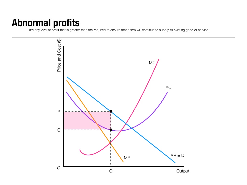automatically implies picking a price P. Why? Because the firm must be operating on the demand curve. Any chosen price corresponds to a specific quantity that consumers will buy at that price, and any chosen quantity corresponds to a specific price that will induce consumers to buy the chosen quantity. To sell more, the firm must lower its price.

Graphically, TR is represented the pink rectangle created by P and Q, where abnormal profits are earned (normally described as Super Normal Profit or SNP).

Marginal revenue is the change in total revenue from increasing quantity by one unit.

That is, MR = ∆TR/∆Q, where the change in Q is usually one unit of output.

Now, you might think that MR must be equal to the price, P, because that’s how much you get paid for selling one more unit. But this is not true in general. Why not? Because if you face a downward-sloping demand curve, you have to lower your price to sell more.

So if you increase your quantity, you’re also lowering your price for all the previous units of the good.

Example: Suppose you’re currently selling 10 units at £20 each. To sell an 11th unit, you’ll have to lower the price to £19. So, you gain £19 from the additional unit. But you also lose £1 each on the previous ten units that you could have sold at £20 each. So your marginal revenue from the 11th unit is not £19, but rather £9.

You can see this from looking at the total revenue: before, TR = 20x 10 = 200, but now TR = 19 x 11 = 209. Thus, TR rose by only £9.

This analysis leads to the following general conclusion: that MR is always below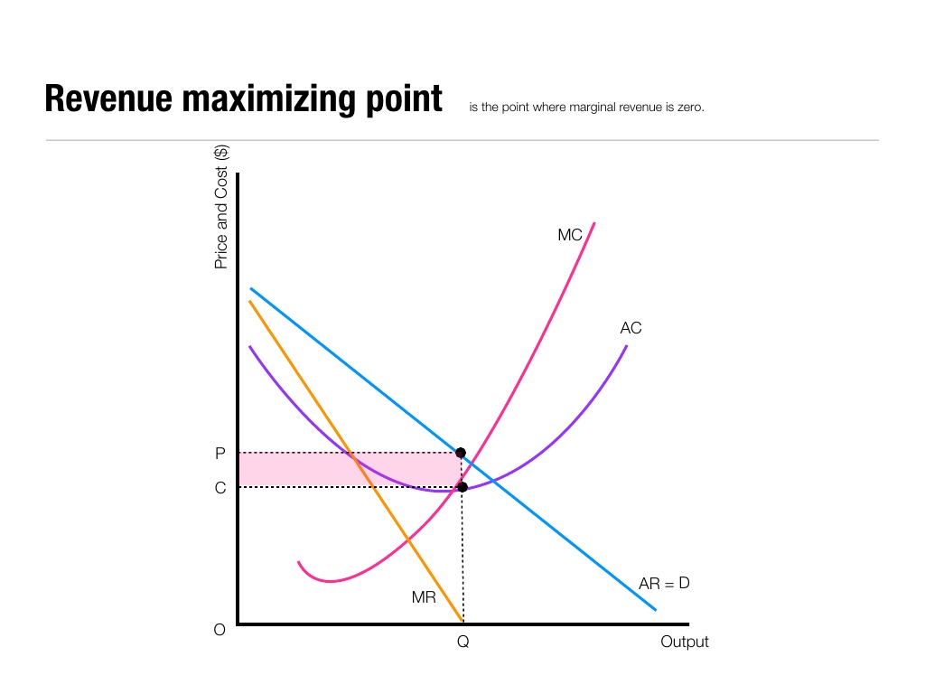 the demand curve. Why? At any quantity, the demand curve tells us the price corresponding to that quantity. But we’ve just shown that the MR must be less than the price, and hence below the demand curve. The only place MR and the demand curve are equal is the point where they cross the vertical y axis. And where MR cuts the x axis we have the revenue (not profit) maximising output (see diagram). Notice profit is still posiitve (the pink block) but not as large as before.

In general, any time a firm lowers its price, there are two effects: the “people buy more units” effect, and the “people pay less per unit” effect. Which effect is larger determines whether MR is positive or negative. It turns out this is closely related to the price elasticity of demand.

A Digression: Price Elasticity of Demand

Elasticity refers to the degree of responsiveness of one variable to another. It’s not enough to say, for instance, that a rise in price leads to a fall in quantity demanded (the Law of Demand); we want to know how much quantity changes in response to price.

A simple way to see the degree of responsiveness is simply to look at the slope. A flatter demand curve represents a greater degree of responsiveness (for a supply or demand curve), as shown in the above graphs: the flatter demand curve produces a larger change in quantity for the same change in price.

Using just the slope is the quick way to think about elasticity. The extremes are easy to remember: A perfectly elastic demand curve is horizontal, because an infinitely small change in price corresponds to an infinitely large change in quantity; the graph looks like the letter E for elastic. A perfectly inelastic demand curve is vertical, because quantity will never change regardless of the change in price; the graph looks like the letter I (for inelastic).

But using the slope can be misleading, because it doesn’t tell us the significance of the quantities. Suppose a £1 increase in price leads to almost everyone choosing not to buy the good. That would not surprise us for chocolate bars, but it would certainly surprise us for televisions. The point is that a £1 increase is not much relative to the total price of TVs, but it is huge relative to the total price of chocolate bars. This is why we use elasticity instead of just the slope.

Definition of price elasticity of demand: the percentage change in quantity demanded divided by the percentage change in price. That is,

Ed = %∆Qd/%∆P

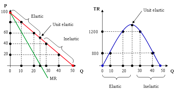When the demand curve is a straight line, as in the diagram above, the MR always has a slope exactly twice that of the demand curve, so that it crosses the horizontal axis exactly half-way between the origin and the point where the demand curve does crosses the axis. Why? Because it turns out that a linear demand curve is always unit elastic exactly half-way down its length, and therefore MR crosses the horizontal axis at a quantity exactly half-way down the demand curve. And recall again a fundamental mathematical relation:

When MR = 0, TR is at its highest point.

The Profit-Maximizing Decision

The firm uses MR and MC to decide how much to produce.

• Suppose increasing output by one unit will bring in more additional revenues than it costs to produce. That is, MR > MC. Then it makes sense to produce the unit, because doing so will create more added benefit than added cost.
• On the other hand, suppose your last unit cost more to produce than it brought in additional revenue. Then MR < MC. And it makes sense to cut back your production (not produce that unit after all), because the last unit created more added cost than added benefit.
• So the only point at which you’re satisfied is where MR = MC. This is the general rule for profit maximisation, which we’ll use with any firm, whether a perfect competitor, monopolist, or anything in between.

Graphically, we find the quantity Q where the MR and MC curves cross. What price corresponds to this quantity? We find it by extending Q up to the demand curve to and reading off P from the y axis. No other price will work: a higher price will reduce sales below Q, and a lower price will increase sales above Q.

How much profit does the firm actually make? To find this out, we need more information about the firm’s costs. We can get all the information we need from AC.

Recall that AC = TC/Q. Therefore, TC = AC×Q. Graphically, we can see this as the pink rectangle created by Q and AC on the AC curve.

Profit is defined as the difference between TR and TC. TR, as we saw before, is the pink rectangle defined P x Q. TC is the rectangle AC x Q. So the difference in the areas of these rectangles is profit, as shown above.

As drawn, the firm is making profits, but it needn’t be such a happy outcome. If the AC curve had been higher, we could have arrived at AC greater than the price. When this happens, the firm is making losses. This can happen even though the firm is doing the best it can, because any choice other than Q would make it lose even more (with the possible exception of shutting down entirely – something we’ll take up later).

The Profit Function

The MC – MR approach yields the same optimal quantity that you would get if you looked directly at a profit function. A profit function simply shows how much profit you make at each level of output.

The very highest point on this curve occurs at Q, which is also exactly the 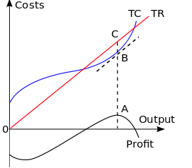quantity at which the MC and MR cross. If we express this in terms of total curves, it is the output where TR is greatest distance from TC. As the marginal curves are the slope of the total curves, it is also the output at which two lines drawn tangential to TR and TC are parallel, as the diagram illustrates, point A of maximum profit corresponds to B and C.

 Applications of MC = MR

The MC = MR rule is a very versatile one, which can be applied to many other decisions by firms other than how much to produce. It can be applied to hours of operation: stay open as long as the added revenue from the additional hour exceeds the cost of staying open another hour. Or it can be applied to advertising: increase the number of times you run your TV commercial as long as the added revenue from running it one more time outweighs the added cost of running it one more time. Assuming there is a constant price per 30-second commercial, the situation might look like this:

 

This is just one of the many ways in which MR = MC rule can be used to make business decisions other than choosing the profit-maximizing quantity.

Also, notice that average cost did not play any role in the choice of output. All that matters is the marginal effect on profits of increasing or decreasing your output. If a firm fails to follow the MC = MR rule and uses average cost instead, it will lose profits.

The case of Continental Airlines

An airline has to decide how many flights to run during any given period of time. In the early 1960s and before, airlines typically made this decision by asking whether the additional revenue from a flight (the MR) was greater than the per-flight cost of a flight. In other words, they used the rule MR = TC/Q. But Continental broke from convention and started running flights even when the added revenues were below average cost. The other airlines said Continental was crazy – but Continental made money hand over fist. Eventually, the other airlines followed suit. What made Continental’s strategy superior?

The per-flight cost consists of variable costs, including jet fuel and pilot salaries, 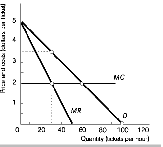and those are very relevant to the decision about whether to run another flight. But the per-flight cost also includes expenditures like rental of terminal space, general and administrative costs, and so on. These costs do not change with the number of flights, and therefore are irrelevant to that choice. The MC is a straight line,a s in the diagram (although ignore the axes here as we are talking about more than just ticket sales in this example).

In order to put MC – MR thinking to its greatest use, we need to adopt a broader notion of fixed and variable inputs. So far, we’ve thought about them in terms of time: variable inputs can be changed in a given period of time, while fixed inputs can’t. But a better way of thinking about them is in terms of “the meeting you’re at” – that is, what kind of a decision are you trying to make? Some inputs are fixed with respect to some decisions, while they are variable with respect to others. For whatever kind of decision you’re making, only the inputs that are variable with respect to that decision are relevant.

Example: Airlines again. When the airline is deciding whether to run an additional flight, the costs of G&A, reservation systems, etc., are fixed. The costs of jet fuel, pilots’ wages, meals, flight attendants’ wages, etc., are variable.

But now suppose the airline has already decided to run a particular flight, and now they’re deciding how many seats to sell (that is, what price to charge per seat).

For this decision, the costs jet fuel and pilots’ wages are fixed, while only the costs of meals and flight attendants’ wages (assuming more customers require more flight attendants) are variable.

Example: If you’re deciding how many hours your employees should work, their wages are variable costs, but their fixed benefits packages (e.g., health insurance)are fixed costs. If you’re deciding whether to hire a new employee, both wages and benefits are variable costs.

The Shut-Down Decision

There is one exception to the rule that average costs are irrelevant in deciding how much to produce: the decision about whether to produce at all.

You should think about the MC = MR rule as the rule you should follow if you’vedecided to produce at all. But it might make sense to shut down the firm instead. How should the firm make this choice? You might think that the firm should shut down if it’s making losses, but that’s not quite true. Why? Because even if the firm shuts down, it will still have to pay its fixed costs (in the short run). So what really matters is whether the firm’s revenues cover its variable costs. If the answer is yes, the firm should stay open even though it’s making losses – because its revenues still partially offset the fixed costs. But if the answer is no, the firm should shut down – because the choice to produce is just adding even more losses on top of the fixed costs.

In other words, it must be the case the firm’s total revenues (TR) exceed the firm’s total variable costs (TVC).

TR > TVC

P×Q > AVC×Q

P > AVC

This shows that the firm should stay open if the price (at its optimally chosen quantity) is greater or equal to its average variable cost. But if the price is below the average variable cost, the firm should shut down.

Note that this is a short-run shut-down decision. In the long run, there are no fixed costs, only variable costs. That means the firm can avoid making any losses at all by shutting down, so the firm should shut down any time it’s making economic losses — unless there are changes the firm can make to its scale that allow it to escape those losses. This may be possible because the firm can shift to a different SRATC curve via a different capital choice.

The firm would need to invest in new capital and thereby change its total cost structure and hence the shape and position of the AC curve.