Aggregate Demand

The level of economic activity is explained by changes in key expenditure items within the Aggregate Demand (AD) equation – consumption, investment, government expenditure and net exports (X-M). Remember that from the idea of the circular flow (core macroeconomic concept 1) we derived the AD equation (core macroeconomic concept 2).

In the Keynesian model, a fall in one or more of these types of expenditure was shown by a downward shift in the AMD curve. If the fall in AD is significant, we experience an economic downturn as real GDP falls. Increases in expenditure, on the other hand, are shown as an upward shift in the AD curve. Equilibrium levels of output, income and expenditure are higher – an economic upswing or rise in real GDP.

An alternative way of showing macroeconomic activity is to use the AD/AS model which includes changes in the price level (inflation) which the Keynesian model excludes.

Here and in the section on aggregate supply, we introduce this alternative model (the aggregate demand / aggregate supply model) to analyse the fluctuations in economic activity that take place during the business cycle.

The aggregate demand (AD) curve

The aggregate demand (AD) curve shows the relationship between the price level and the quantity of real GDP demanded by households and firms. The relationship between aggregate demand and the price level is negative (inverse), for three reasons.

1. Wealth effect As the price level changes, the real value of money balances held by households also changes. For example, if the price level rises, the purchasing power of your income goes up. To illustrate, imagine you had £20 to spend today -what could you buy? If all prices rise by 20 per cent tomorrow, you are able to buy fewer goods and services. The price level affects my real spending power.

2. Monetary effect Higher price levels means households and firms need to hold more funds to finance their transactions. They could do this by withdrawing money from banks, borrowing, or selling financial assets such as bonds. The rising demand for money drives interest rates upwards, increasing the cost of borrowing, and acting as a disincentive to spending.

3. International effect The domestic price level rises relative to other countries, domestic goods and services become less competitive in those countries. Other things being equal, this means there will be an increase in imports and a fall in exports.

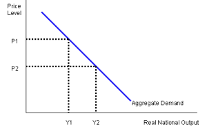
If the price level rose from P2 to P1 below, households and firms will reduce their aggregate demand for goods and services to a lower level, shown as a movement along the AD curve following from a change in the price level.

Movements along the AD curve

A change in the price level in the economy will result in a movement along the AD curve. for example, in the diagram here a fall in the price level from P1 to P2 results in a rise in real GDP (Y1 to Y2). However, a change in any of the elements of aggregate expenditure (C,I,G,X or M) will bring about a shift of the entire aggregate demand curve .

Aggregate purchasing power alters if the price level changes. An increase in prices would mean that real purchasing power falls. Falling real purchasing power represents a movement along the aggregate demand curve. Any change in the price level in the economy will result in a movement along the AD curve.

Conclusion: the AD curve plots real output against inflation and shows the effect of rising or falling prices on aggregate output.

Shifts in AD curve

1. Consumer Spending

Aggregate consumption is influenced by disposable income, stock of wealth, interest rates and expectations. there are a number of factors which could change the willingness of households and firms to spend.

Here are three:

• changes in interest rates
• changes in taxation levels
• changes in expectations and confidence (of consumers or business)

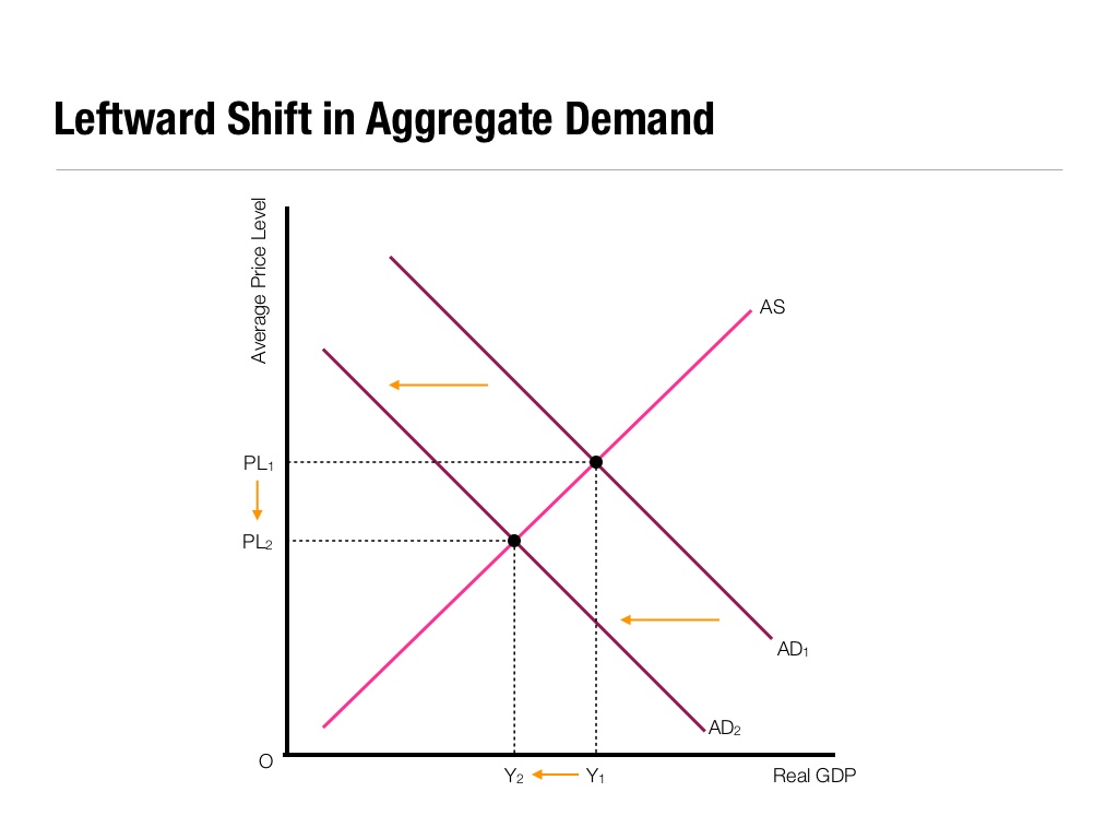
Assuming there is no change in the price level at the same time, if any of these three variables changes then the whole AD curve would shift, either inwards to the left (bringing about a fall in real output as in the diagram here) or outwards to the right (bringing about an increase in real output). For example, if interest rates go up there is a reduction in aggregate demand (because the cost of borrowing rises) or because expectations about the future worsen.

The rate of interest represents the opportunity cost of consumption: higher interest rates mean that more interest is given up for every pound spent.

2. Investment

Investment is influenced by levels of retained profit, interest rates, and expectations. A fall in business expectations would reduce the willingness of businesses to invest and  AD will shift to the left.

3. Government Spending

An increase in Government Spending will, ceteris paribus, shift AD to the right.

4. Net exports – the trade effect (X-M)

Net exports are influenced by domestic and overseas economic activity, tariffs, quotas, exchange rates, terms of trade.

A depreciation in the exchange rate would make exports more competitive, and reduce the competitiveness of imports. Hence AD shifts to the right as (X-M) generates a net injection into the circular flow.

Comparative growth rates are a critical factor in determining our trade balance. If the UK is growing faster than our trading partners. UK demand for imports (M) is likely to grow faster than overseas demand for UK exports (X). The AD curve will shift inwards, ceteris paribus, as (X-M) creates a negative effect on real GDP (or net withdrawal from the circular flow).