Long-Run Production

In the short run we analyse marginal and average product which exhibits the law of diminishing marginal returns. But what happens when all factors are variable? Again we apply the idea of rationality: rational producers are assumed to be cost-minimisers. They will tend towards Minimum Efficient Scale, where opportunity costs are at their lowest.

source: cuny

So far, we’ve taken capital (K) as fixed. But in the long run (LR), firms can choose their level of capital. In the LR all inputs (Land, Labour, Capital) are variable. As a result, all costs are variable costs. There are no fixed costs in the long run.

When the firm is able to vary all its inputs, it must choose a combination of inputs to produce its chosen level of output. There may be many combinations of inputs that can produce the same amount of output. So the cost-minimizing firm must pick the input combination that produces its chosen level of output at the lowest cost.

From this point forward, when we are talking about firms operating in the LR, we will assume they are minimising their input costs as part of our rationality assumption.

So, what does this do to the firm’s cost curves? Let’s take them in turn.

Total cost is still fixed cost plus variable cost. But in the long run, FC = 0. How will the LRTC compare to the SRTC? It turns out that for any quantity, LRTC must be less than or equal to SRTC. Why? Because in the long run, the firm can choose a cost-minimizing input combination, which it cannot do in the short run. It certainly has the option, in the long run, of choosing the exact same level of capital and labour as it did in the short run, so it couldn’t possibly do worse. But it can usually do better by altering the combination of capital and labour.

K	L	TC
1	16	106
2	8	68
4	4	64
8	2	92
16	1	166

Average total cost is still defined as total cost divided by quantity. LRAC = LRTC/Q. Like SRAC, it will typically be U-shaped. Just as LRTC was always less than or equal to SRTC because of our assumption of cost-minimisation, LRAC is always less than or equal to SRAC for the same reason.

Note that SRAC is always greater than or equal to LRAC. What’s happening at the one point where SRATC = LRATC? That’s where the amount of capital (fixed inputs) the firm happened to have in the short run is exactly the same amount of capital (fixed inputs) the firm would choose to have in the long run, if it wished to produce that quantity.

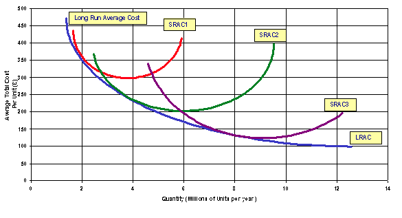
In the above, we have been acting like there is just one SRAC, but we could draw more. The one we drew was based on some fixed level of capital, which implied a particular level of fixed costs. But what if the firm had a different fixed level of capital in the short run?

Then we could construct a different set of short-run curves based on that 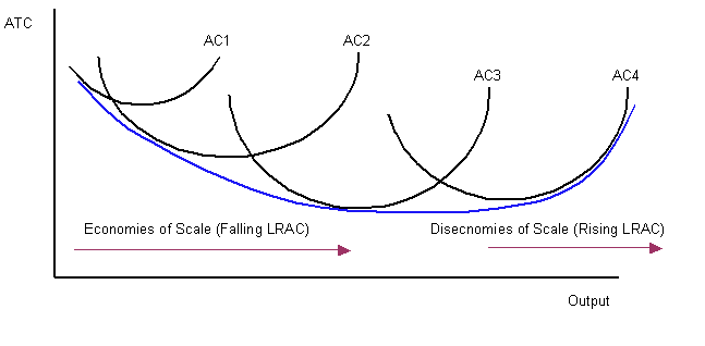assumption. We could do this for any level of fixed inputs that a firm might have, so we could really have an infinite number of SRAC’s. If we kept on drawing in more SRACs, we would eventually find that the LRAC forms an envelope of them all (encompassing them all from below). Hence the name ‘envelope curve’.

We can also talk about long-run MC (or LRMC). It is calculated just like short-run MC, except we find the change in LRTC instead of short-run TC. It tells you how much it costs to increase output by one more unit, assuming that you’re able to adjust your combination of inputs optimally.

Economies and Diseconomies of Scale

In the above diagrams we have assumed a certain type of technology – specifically, a technology that results in a U-shaped LRAC curve. That means average costs decline over some range of production, but eventually start rising again. Why? What have we assumed here?

Notice that the shape of the LRAC and SRAC are similar. But the reasons are different. The SRAC’s U- shape resulted from changing average product of labour, combined with fixed cost spreading. The SRAC falls because of increasing average product of labour and fixed cost spreading, and it eventually rises because of decreasing average product of labour – the law of diminishing marginal returns applies. But the LRAC’s shape is related to returns to scale.

The lowest point of a LRAC curve is called the minimum efficient scale. The minimum efficient scale (MES) is the output for a business in the long run where the internal economies of scale have been fully exploited. It corresponds to the lowest point on the long run average total cost curve, point A in the diagram, and is also known as the output of long run productive efficiency. Hence, the MES achieves production of a good at the lowest possible opportunity cost, which means at this quantity the production involves foregoing the least amount of other goods.

Economies of scale occur when output increases proportionally more than cost increases. E.g., you can double output by less-than-doubling cost. Economies of scale occur mainly because of specialisation – not just specialisation of workers among tasks, but also specialisation in capital usage. A greater amount of capital may allow better specialisation, because the capital can be catered to their specific tasks. Economies of scale usually accompany mass production techniques (which is really just another way of saying “specialisation combined with appropriate capital”) and are depicted by points to the left of the MES.

Other reasons that economies of scale occur:

(a) Lower inventory (unsold stock) costs. Inventory is maintained in order to reduce the likelihood of running out if quantity demanded is higher than average. Small-scale firms are likely to experience greater variance in their sales, which means they need to keep relatively high inventories when measured as a fraction of sales. A large-scale firm will experience less variance in its sales, and thus can get by with a smaller ratio of inventories to sales. Many large supermarkets operate a ‘just in time’ strategy of stock holding.

(b) Physical properties of production. Sometimes the physical nature of the production process implies a falling ratio of cost to output at output increases. For example, as the radius of a pipeline increases, the surface area (which determines the amount of metal required) increases as a linear function of radius (circumference = 2ðr) while volume increases as a function of the square of the radius (area = ðr2).

(c) Volume discounts, resulting from contract-writing savings or the greater buying power of a larger purchaser.

(d) Marketing advantages. A larger scale firm with more outlets is more likely to benefit from a given amount of advertising, because each viewer will be more able to act on the desire encouraged by the ad.

Diseconomies of scale occur when output increases proportionally less than cost increases. This happens when the benefits of specialisation and mass production begin to be overwhelmed by the costs of large-scale activity: layers of management, difficulty of communication, problems with monitoring, etc.

Other reasons diseconomies of scale occur:

(a) Large-scale firms often pay higher wages, in part because their workforces are more likely to be unionized, in part because they may have to pay compensating differentials to overcome a taste workers have for working in smaller firms.

(b) Spreading specialised resources too thin. Some resources are unique, and thus cannot really be scaled up in the scaling-up process. For instance, if a firm’s biggest asset is its very clever owner, that owner cannot be duplicated, and his attention may get spread too thin as the firm grows in size.

Economies and diseconomies of scale correspond to the downward-sloping and upward- sloping portions, respectively, of the LRAC curve. This is apparent from their definitions. Economies of scale means Q increases at a higher rate than LRTC, so LRTC/Q must decline, and vice versa for diseconomies of scale. In addition, a LRAC may have a flat section in the middle; this section corresponds to constant returns to scale.

Could we have made different assumptions about technology? Certainly. For example, we could have assumed never-ending economies of scale (see above), which implies an always downward-sloping LRAC curve. Karl Marx believed that all major industries were like this, and predicted for that reason that all industries would end up being monopolies. The USSR agreed that all industries must have downward-sloping LRAC’s, and that’s why they consolidated all their industries into massive plants. But history has shown this to have been a poor choice. However, there are some industries, especially certain utilities, that do seem to have this feature. We call such industries natural monopolies.

The textbook uses the term “economies of scale” to refer to any decrease in ATC (thus, to any downward-sloping portion of an ATC curve), regardless of the time period. As I indicated earlier, this is an error of terminology. However, there is a good argument from a real-world perspective for the textbook’s approach. For many industries, there will be some inputs that will remain fixed for a very long period of time – for instance, the number of power generators operated by an electric utility. So by the usual economist’s definition of terms, the firm is not really in the long-run in the meantime, and thus scale economies don’t apply (the term “scale” being reserved for situations in which all inputs are variable).

But there are many variable inputs besides labour, and the firm can use the process of cost minimization to choose the optimal combination of the variable inputs.

As a result, many of the lessons of economies of scale apply even in situations where some inputs are fixed for the time being.

Economies of Scope

Economies of scope exist when a firm can produce two or more products at lower cost than the two products could be produced separately. One way to represent this mathematically is like so:

There are two basic reasons this may occur. First, a positive level of production of one good (x) may lower the marginal cost of producing another product (y).

Second, some fixed inputs can be shared between the two production processes, thereby allowing greater fixed-cost spreading. (Notice that economies of scope is not, like economies of scale, a purely long-run concept.)

Some more specific reasons why economies of scope occur:

(a) Volume discounts. As discussed in the section on economies of scale, purchasing in bulk can lower transaction costs. A firm might not need to produce enough of a single good to justify a large purchase, but if two or more goods share some of the same inputs, then purchasing in bulk can make sense.

(b) Marketing advantages. If a single producer makes multiple products, the same amount of advertising can benefit all the product lines. For example, if McDonald’s runs an advertisement, it can benefit all the food products associated with McDonald’s. This is called “umbrella branding.”

(c) Research and development spillovers. The research done on one product can generate discoveries relevant to other products. For example, research on new paint thinners might yield results useful for nail polish removers, carpet cleaners, and so on.

The Learning Curve

The learning curve represents the fact that a firm’s costs of production tend to fall as the firm gains more experience in the production of its product. The usual picture shows a downward-sloping curve as a function of the firm’s cumulative production.

People often confuse the learning curve, shown above, with an average (total or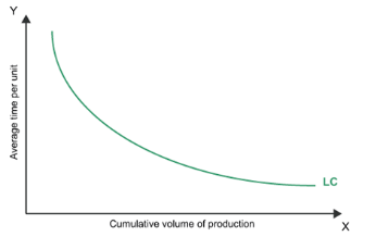 variable) cost curve. But they are quite different. Both curves show a firm’s average cost of production for some product. But the ATC curve shows the firm’s average cost of production at a fixed point in time, i.e., for a fixed level of experience, at many different quantities of output. The learning curve, on the other hand, shows the firm’s average cost of production at a fixed level of output for many different levels of experience. Notice that the horizontal axis is “Cq,” meaning cumulative quantity – the total amount of production the firm has accomplished over its lifetime. Cumulative quantity is usually a good proxy for the firm’s experience.

In some books, you’ll find a graph showing the relationship between the learning curve and the average cost curve. In order to show the relationship cleanly, the authors have assumed constant returns to scale, which imply horizontal long-run ATC curves. The important point is that, as time passes and experience accumulates, the firm’s long- run ATC changes, usually for the better – and that’s true whether or not there are economies (or diseconomies) of scale.

In general, we assume (for simplicity) that the learning effect lowers average cost at every level of output. But it’s possible for the learning effect to impact only average cost at certain levels of output, specifically, the levels of output the firm has had experience with.